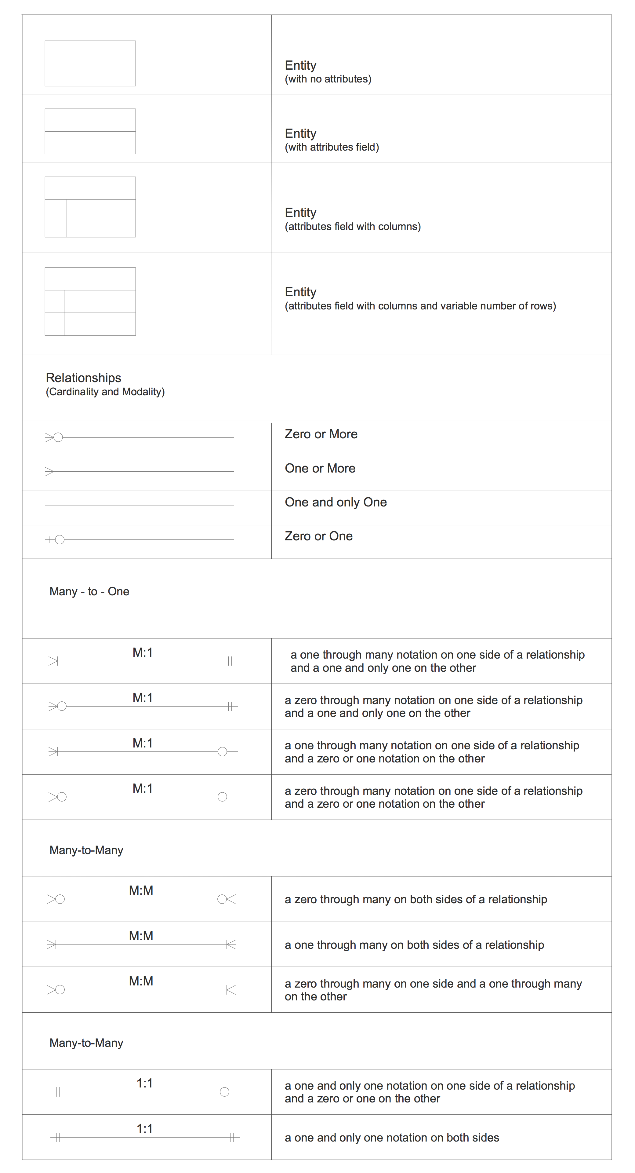
Relational model
The relational model specifies a mathematically grounded way to store, organize, and manipulate data in a set of tables (relations, which also comprise views and sequences). The schema specifies the names, data types and constraints of the columns (fields) that make up the table, and the actual data are the rows (records) filling it. This model is the foundation of how relational databases persist data.
A conceptual schema is a high-level design of entities (any recognizable objects in the real world) and their relationships, whereas a physical schema is a database-specific design focused on the implementation of the conceptual schema.
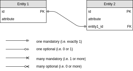
Usually, different kinds of entities are modeled through separate tables, and each row represents an entity instance. A relationship describes a connection between these entities (e.g. between customers and orders, and between orders and products), more physically by cross-referencing columns using primary- and foreign-key constraints. The cardinality of such a relationship specifies the number of objects on each side of the relationship, and modality indicates whether a relationship is optional or required.
-
One-to-one relationships are implemented by means of a unique foreign key.
-
One-to-many relationships are implemented by a non-unique foreign key, where the many-side will have a foreign key identifying the one-side.
-
Many-to-many relationships are implemented as a cross-reference table T3 that uses two foreign keys, to primary key of T1 and primary key of T2, together forming the primary key of T3.
Visualization: Crow’s Foot Notation
Keys
Keys are specific kinds of constraints (i.e. rules on what kind of data is allowed in a column) and as such part of the schema definition. Their main purpose is to ensure data integrity in the sense that data records can be uniquely identified and referenced.
Primary keys
A primary key is a collection of one or more columns that uniquely identifies each row in a table. In other words, the constraint PRIMARY KEY is the same as NOT NULL UNIQUE.
Each relational table can have only one primary key. When a primary key is created, also an index is created, that facilitates data selection and sorting based on the primary key column.
Keys can be natural, i.e. one or several columns that happen to be unique, or more likely surrogate, i.e. created for the specific purpose of being a unique identifier, such as auto-incrementing integers or UUIDs.
Foreign keys
A foreign key is a column that refers to the primary key of another table, thereby acting as a cross-reference between tables. Foreign key columns obviously need to have the same data type as the primary key column of the other table, and in most DBMS the foreign key constraint also prevents foreign key values that don’t exist as primary key value (referential integrity).
As opposed to primary keys, foreign keys don’t need to be unique, can be NULL, and there can be arbitrarily many of them in one table.
A column can be both a primary and a foreign key.
Normalization
The goal of normalization is to design the schema in a way that it avoids or at least minimizes anomalies, mainly by distributing information across separate tables.
- Update anomaly: If data is duplicated, updating it in one place while not updating it in another leads to inconsistencies, e.g. leading to different answers to a query that should only have one.
- Insertion and deletion anomaly: When storing particular information only together with other information, e.g. contact details in an events table, then that information is not available independently, i.e. it can only be inserted when other information is inserted, and is lost when that other information is deleted.
PostgreSQL
Basic commands
Lists all databases and exit:
$ psql -l
Connect to database:
$ psql hero-database username
Or via postgres terminal:
$ sudo -i -u postgres
$ psql
postgres=# \l
postgres=# \c hero-database
hero-database=#
Command line
| Command | Description |
|---|---|
createdb demo |
creates a new database called demo |
dropdb demo |
deletes the database called demo |
psql -d demo |
start a psql session, connecting to the database demo |
PostgreSQL console
| Command | Description |
|---|---|
\l, \list |
display all databases |
\c demo |
connect to database demo |
\dt |
display all tables of the current database |
\d books |
show the schema of the table books |
\? |
list of console commands |
\h |
list of SQL help options |
\q |
quit |
Importing and exporting data
Importing from SQL file:
Command line:
$ psql -d demo < dump.sql
psql console:
# \i /path/to/dump.sql
Importing from CSV file:
psql console:
# \copy table          from 'table.csv' with CSV HEADER DELIMITER ',';
# \copy table (c1, c2) from 'table.csv' with CSV HEADER DELIMITER ',';
\copy invokes the corresponding SQL command COPY:
COPY table               FROM 'absolute/path/to/table.csv' WITH CSV HEADER DELIMITER ',';
COPY table (name, color) FROM 'absolute/path/to/table.csv' WITH CSV HEADER DELIMITER ',';
Note that HEADER just means the first line is going to be ignored;
the headers are not used for matching with the table columns.
So if the order of columns in the CSV differs from the order of columns
in the table schema, the columns have to be specified in the correct order
in the COPY statement.
Exporting a database or a specific table into an SQL file:
Command line:
$ pg_dump -d demo [-t table] [--inserts] -f dump.sql
Data types
Data types are used by databases to decide how much memory to allocate to the values, how to perform operations and calculations on them, and how to sort them.
Serial
serial is a notational shortcut for creating a sequence:
CREATE TABLE items (
  id serial
);

-- is interpreted as:
CREATE SEQUENCE items_id_seq;
CREATE TABLE items (
  id integer NOT NULL DEFAULT nextval('items_id_seq')
);
Sequences are a special kind of database object designed for generating auto-incrementing unique numeric identifiers, usually used for artificial primary key columns. Sequences consist of a single-row table with a value of type bigint together with information on the sequence, as well as a generator for incrementing the numeric value. The value can be accessed using nextval('sequence_name') and currval('sequence_name'), and can be set using setval('sequence_name', value).
# select * from items_id_seq;

 sequence_name | last_value | start_value | increment_by |      max_value      | min_value | cache_value | log_cnt | is_cycled | is_called
---------------+------------+-------------+--------------+---------------------+-----------+-------------+---------+-----------+-----------
 items_id_seq  |          1 |           1 |            1 | 9223372036854775807 |         1 |           1 |       0 | f         | f

# select nextval('items_id_seq');

 nextval
---------
       1
(1 row)

# select nextval('items_id_seq');

 nextval
---------
       2
(1 row)
Start and incrementing value (default 1) as well as other options (such as min and max values) can be specified explicitly, e.g.
CREATE SEQUENCE id_seq
START WITH 10
INCREMENT BY 2;
Decrementing sequences can be created by specifying INCREMENT BY -1.
A sequence can also be dropped like any other table:
DROP SEQUENCE id_seq;
An alternative for unique identifiers are UUIDs:
uuid, e.g.a0eebc99-9c0b-4ef8-bb6d-6bb9bd380a11
Numerical values
-
integer(alias:int) -
real, with variable precision and special valuesInfinity,-Infinity,NaNBeware that not all floating point numbers (like
pi()) can be stored exactly, so the binary arithmetic performed on them can lead to errors. For example,1.0 - 0.2 - 1.0 + 0.2withreals likely will not end up to be0but something like5.551115123125783E-17. Therefore, floating point numbers should never be used to store information where exact values are needed (e.g. money). -
numeric(alias:decimal),numeric(precision, scale), ornumeric(precision)withscale = 0numeric(4, 2)are precise values with (up to) 4 digits, 2 of which after the decimal point, e.g.23.55or4.7or10. Values with more digits after the decimal point are rounded, e.g.4.798is stored as4.80. Withnumerics,1.0 - 0.2 - 1.0 + 0.2equals to0, as expected.
Strings
char(fixed-length)varchar(max-length)text(orclobfor character large object) for textual information of any length
Strings are always enclosed by single quotes.
'some string'
'A long and winding road'
'That wasn''t a good idea'
'"Indeed!"'
Double quotes can be used to escape identifiers that are reserved keywords in SQL, e.g. "when".
When filling an char(n) field with a string shorter than n characters, it will be filled up with spaces.
When trying to fill it with a string that is longer, an error is thrown (except when the excess characters are all spaces, in this case the string is truncated to the expected length).
If there is an explicit typecast to char or varchar and the string is longer than the provided length value, the string will be truncated to that length, e.g. 'too long'::varchar(5) gets 'too l'.
Date and time
dateas'yyyy-MM-dd', e.g.'2017-08-20'timeas'hh:mm:ss', e.g.'17:00:00'timestampas'yyyy-MM-dd hh:mm:ss', e.g.'2017-08-20 17:00:00'
Incomplete timestamps will be filled up automatically, e.g. '2017-08-20' becomes '2017-08-20 00:00:00', and '2017-08-20 17:00' becomes '2017-08-20 17:00:00'. Thus, a condition to include all timestamps in 2017 would be: t BETWEEN '2017-01-01' AND '2018-01-01'.
Dates, times, and timestamps can be compared using the numerical comparison operators (<, =, BETWEEN, etc.).
time and timestamp have variants that include timezone information, e.g. '2017-8-20 17:00:00+02' with an 2-hour offset from UTC.
Boolean
boolean
Values can be TRUE, FALSE, or NULL (unknown).
Type casts
CAST (expression AS type)
expression::type
SQL
SQL (Structured Query Language) is a special-purpose, declarative programming language to interact with relational databases.
The SQL vocabulary is categorized into three sub-vocabularies:
-
The Data Definition Language (DDL) is a vocabulary for specifying the database schema, in articular for creating, modifying and deleting databases, tables, and constraints. This comprises all SQL commands that define the structure and properties of data but don’t actually manipulate any data records, such as
CREATE,ALTER, andDROP. (The latter is partly also DML, as dropping a database also deletes all data records in it.) -
The Data Manipulation Language (DML) is a vocabulary for managing data, i.e. for retrieval of data records (querying) and manipulation of data records (inserting, modifying, deleting). Also known as CRUD, the four basic functions of persistent storage: * Create data (
INSERT) * Read data (SELECT) * Update data (UPDATE) * Delete data (DELETE) -
The Data Control Language (DCL) is a vocabulary for controlling rights and roles for accessing data. This comprises in particular
GRANTandREVOKE.
Adher to the SQL style guide.
SQL: Data Definition Language (DDL)
Creating and dropping tables
CREATE TABLE table_name (
    PRIMARY KEY (column1),
    column1 <datatype> <column_constraints>,
    column2 <datatype> <column_constraints>,
    <table_constraints>
);
Addind and dropping a column:
ALTER TABLE table ADD  COLUMN column <datatype> <constraints>;
ALTER TABLE table DROP COLUMN column;
Dropping tables and databases:
DROP TABLE table_name [ , other_table_name ];

DROP DATABASE database_name;
Constraints
The database schema can be used to restrict data injection in three ways:
- datatype
- modifiers (column constraints)
- table constraints
| Modifier | Constraint |
|---|---|
NOT NULL |
CHECK (column IS NOT NULL) |
UNIQUE |
UNIQUE (column) |
UNIQUE (column1, column2, ...) |
|
DEFAULT value |
- |
PRIMARY KEY |
PRIMARY KEY (column) |
PRIMARY KEY (column1, column2, ...) |
|
REFERENCES other_table (column) |
FOREIGN KEY (column) REFERENCES other_table (column) |
CHECK condition |
CHECK condition |
Constraints can be explicitly named by prefixing CONSTRAINT constraint_name ....
Options for foreign keys:
ON UPDATE CASCADEON DELETE CASCADEON DELETE SET NULLON DELETE SET DEFAULT- and others
FOREIGN KEY (c1) REFERENCES table (c2) ON DELETE CASCADE means that if a value in the referenced column c2 is deleted, all rows with that value in c1 are deleted as well. Alternatively, the value in c1 can be set to NULL or the column’s default value.
FOREIGN KEY (c1) REFERENCES table (c2) ON UPDATE CASCADE means that updates of values in c2 are copied to the respective occurrences in c1.
If no options are specified, the default is ON UPDATE RESTRICT and ON DELETE RESTRICT, i.e. updating and deleting values in c2 is not allowed if they are referenced in c1.
If a table has a multi-column primary key, the foreign key would be accordingly multi-column, e.g. FOREIGN KEY (person_first_name, person_last_name) REFERENCES person (first_name, last_name)
Adding a constraint
During table creation:
-- Column constraint as modifier

CREATE TABLE table (
  id    serial       PRIMARY KEY,
  other integer      REFERENCES table (column),
  age   integer      CHECK (age BETWEEN 0 AND 100),
  email varchar(100) CHECK (email LIKE '%@%')
);

-- Table constraint

CREATE TABLE table (
  PRIMARY KEY (id),
  id    serial,
  other integer,
  age   integer,
  year  integer,
  CHECK (age > 0 AND 2017 - age = year),
  FOREIGN KEY (other) REFERENCES table (column)
);
To an existing table:
ALTER TABLE ADD CONSTRAINT name PRIMARY KEY (column);
ALTER TABLE ADD CONSTRAINT name FOREIGN KEY (column) REFERENCES table (column);
ALTER TABLE table_name ALTER COLUMN column [ADD CONSTRAINT name] SET DEFAULT 0;
ALTER TABLE table_name ALTER COLUMN column [ADD CONSTRAINT name] SET NOT NULL;
Deleting constraints
ALTER TABLE table DROP CONSTRAINT constraint_name;

ALTER TABLE table ALTER COLUMN column DROP NOT NULL;
Enums
Either as constraint:
CHECK (column IN ('value1', 'value2', 'value3'))
Or by creating an own data type:
CREATE TYPE weekday AS ENUM('monday', 'tuesday', 'wednesday', 'thursday', 'friday', 'saturday', 'sunday');
DQL: Data Manipulation Language (DML)
Inserting records
INSERT INTO table_name (column1, column2, column3, ...)
VALUES (value1, value2, value3, ...),
       (value1, value2, value3, ...);
NULL is inserted for all columns that are omitted in the INSERT statement.
If all columns are included in their expected order, the column names can be omitted:
INSERT INTO table_name
VALUES (value1, value2, value3, ...);
Updating records
UPDATE table_name
   SET column1 = value1,
       column2 = value2, ...
 WHERE condition;
It is also possible to use arithmetic expressions, e.g. SET price = 2 * price or SET years = years + 1.
Deleting records
Deleting specific records:
DELETE FROM table_name
 WHERE condition;
Deleting all records:
DELETE FROM table_name;
SQL: Querying
Operators
String matching:
LIKE, NOT LIKE
Wildcards:
_matches exactly one character%matches zero or more characters
Boolean:
AND, OR
Set inclusion:
IN, NOT IN
e.g.
WHERE id IN (1, 2)WHERE id IN (SELECT ...)
Comparison:
=, <>, <, <=, >, >=, BETWEEN ... AND ...
In PostgreSQL, a BETWEEN x AND y is equivalent to a >= x AND a <= y, i.e. works for numbers and date times and is inclusive.
If either side of an operator equals NULL, the result will be NULL. This is because NULL refers to a missing or unknown value, so the result of the comparison is also unknown. The same holds for most functions.
Return values that are NULL are not be included in the result set.
Also, NULL values cannot be compared, so in results of statements with ORDER BY clauses rows with NULL values will appear either first or last.
Equality with NULL:
- A condition
column = NULLwill never be true, i.e. the result will always be empty. - A condition
column <> 'some value'will not return rows wherecolumnisNULL. Therefore, in conditions checking forNULL, always useIS NULLorIS NOT NULL. This includes arrays like('value1', 'value2', ...): they cannot containNULL.
Grouping
GROUP BY c groups together all rows that have the same value in column c.
Example:
-- select the number of employees in each department in the year 2013
SELECT department, COUNT(*)
  FROM employees
 WHERE year = 2013
 GROUP BY department;
Columns other than c can have different values within one group, so it makes sense to aggregate on them, but it doesn’t make sense to put them in a SELECT clause without aggregation (which of the values to return?).
GROUP BY column1, column2 groups by (column1, column2), e.g. GROUP BY last_name, first_name.
In addition, groups can be filtered by means of HAVING.
Example:
SELECT last_name, first_name,
       AVG(salary) AS average_salary,
       COUNT(year) AS years_worked
  FROM employees
 GROUP BY last_name, first_name
HAVING years_worked > 2
 ORDER BY average_salary DESC;
Joins
Joins are clause in SQL statements that combine rows from two or more tables, based on a related column between them.
Inner join:
- (INNER) JOIN contains all records in the intersection of both tables.
SELECT *
  FROM table1
       JOIN table2
         ON table2.table1_column = table1.column
 WHERE ...;
This can get as complex as necessary:
SELECT *
  FROM table1
       JOIN table2
         ON table2.table1_column = table1.column
       JOIN table3
         ON (table3.column1, table3.column2) = (table1.column1, table1.column2)
       ...
 WHERE ...;
Outer joins:
- LEFT (OUTER) JOIN contains all records in the left table, with matching records from the right table if present (otherwise
NULL). - RIGHT (OUTER) JOIN contains all records in the right table, with matching records from the left table if present (otherwise
NULL). - FULL (OUTER) JOIN combines the results of left and right join. This is particularly useful for including rows from T1 that don’t have a match in T2 as well as rows in T2 that don’t have a match in T1 without needing a full-blown cross join.
Cross join:
- CROSS JOIN corresponds to the Cartesian product and contains all records of the left table matched with each record in the right table.
The cross join is what you get when you SELECT * FROM table1, table2.
An inner join then is like SELECT * FROM table1, table2 WHERE table1.table2_id = table2.id.
CROSS JOIN is generally best suited to generating test data rather than production queries.
Self joins:
A table can also be joined with itself.
Example:
-- all pairs of students that share the same room
SELECT s1.name, s2.name
  FROM student AS s1
  JOIN student AS s2
    ON s1.room_number = s2.room_number
 WHERE s1.id <> s2.id ;
Subqueries
Performance
EXPLAIN sql-statement constructs a query plan and estimates the costs (in terms of system resources) for executing it.
EXPLAIN ANAYLYZE sql-statement in addition executes the query and displays the time needed for planning and execution.
Useful to compare the efficiency of different queries, e.g. usually using sub-queries is much faster than using JOINs.
When it comes to ORDER BY, it makes a big difference whether you look at an unindexed column, on which sorting is pretty costly (as it needs several passes on the table), or an indexed column, for which sorting comes for free because the index already gives you an order (so retrieval actually doesn’t need any additional sorting). For example:
auction=# EXPLAIN ANALYZE SELECT * FROM bids ORDER BY amount;

                                                QUERY PLAN
----------------------------------------------------------------------------------------------------------
 Sort  (cost=104.83..108.61 rows=1510 width=26) (actual time=0.024..0.025 rows=26 loops=1)
   Sort Key: amount
   Sort Method: quicksort  Memory: 27kB
   ->  Seq Scan on bids  (cost=0.00..25.10 rows=1510 width=26) (actual time=0.004..0.005 rows=26 loops=1)
 Planning time: 0.059 ms
 Execution time: 0.037 ms

auction=# EXPLAIN ANALYZE SELECT * FROM bids ORDER BY item_id;

                                                              QUERY PLAN
---------------------------------------------------------------------------------------------------------------------------------------
 Index Scan using bids_item_id_bidder_id_idx on bids  (cost=0.15..70.80 rows=1510 width=26) (actual time=0.006..0.012 rows=26 loops=1)
 Planning time: 0.058 ms
 Execution time: 0.034 ms
Also, counting is more efficient when done in the database than in the application, because for the latter case, all data to be counted needs to be transfered.
Also, avoid N+1 queries i the application, i.e. queries that are the result of performing an additional query for each element in a collection.
Comments
/* query to retrieve the radius or a circle */
SELECT radius
  FROM circles
 WHERE something      -- fill in condition
   AND something_else -- here as well
Views
A view is a virtual table, created by specifying the query from which is results and a name:
CREATE VIEW view_name
AS <query>
It can then be queried like any other table (SELECT * FROM view_name;), with the only difference that virtual tables are not stored physically: every time data is retrieved from a view, the database re-runs the underlying query.
Views can be deleted as expected:
DROP VIEW view_name;
SQL: Function
Aggregate functions
-
COUNT(*)counts all rows (therefore avoid inLEFT JOINs if you want to only count rows that have values in both tables) -
COUNT(x)counts all rows in whichxis a non-NULLvalue -
SUM(x) -
AVG(x) -
MIN(x) -
MAX(x)
Where x can be any value: column, DISTINCT column, ROUND(column1 / COALESCE(column2, 0)), etc.
Note that NULL as value is ignored.
String functions
-
Concatenation
||, e.g.SELECT 'pi is ' || pi() ;SELECT first_name || ' ' || last_name FROM persons;SELECT id FROM item WHERE lower(name) = 'whatever letters were capitalized';
-
length(column) -
lower(column),upper(column),initcap(column)(first letter uppercase, all other letters lower case) -
substring(column, start_char, number_of_chars)
Numeric functions
+,-,*,/mod(x, y)calculating the remainder ofx/y
Note that / in PostgreSQL is integer division, i.e. 1/4 yields 0 and in order to get 0.25 you have to use decimals (e.g. 1.0/4.0), e.g. by means of casting CAST(column AS decimal).
-
abs(x)for the absolute value ofx -
round(x)for rounding to the nearest integer -
round(x, i)for rounding to a decimal withidecimals (in PostgreSQL this only works whenxis of typedecimal) -
ceil(x)for rounding up,floor(x)for rounding down, andtrunc(x)for rounding towards 0 (i.e. rounding up for negative numbers and rounding down for positive ones)
Date and time functions
current_date,current_time,current_timestampEXTRACT(field FROM column), wherefieldcan beYEAR,MONTH,DAY,HOUR,MINUTE,SECOND, e.g.AT TIME ZONE '...'for conversion to local time, e.g.time AT TIME ZONE 'Europe/Warsaw'-for difference between two timestamps+for moving a date time by an interval (such asINTERVAL '4' HOURorINTERVAL '1' DAY)
The operation - and + are, for example, useful for
- not caring about the specific end date of a month:
date BETWEEN '2010-01-01' AND CAST('2010-02-01' AS date) + INTERVAL '1' MONTH - checking for something within the past
xdays (or hours, or the like):date > CURRENT_DATE - INTERVAL 'x' DAY - checking for something older than 10 years:
birth_date < CURRENT_DATE - INTERVAL '10' YEAR - something around the current time:
time BETWEEN (CURRENT_TIME - INTERVAL '1' HOUR) AND (CURRENT_TIME + INTERVAL '1' HOUR)
Working with NULLs
-
COALESCE(value1, value2, ...)returns the first of the values that is notNULL. This is useful, e.g., for default values during query time, e.g.:SELECT COALESCE(name, 'product ' || id, 'n/a') FROM item;COALESCE(number * 2, 0)Note that both values need to have the same data type, i.e.COALESCE(date, 'no date')will not work and needs to beCOALESCE(CAST(date AS varchar), 'no date').
-
NULLIF(x, y)returnsNULLifxandyare equal, elsex. This is useful, e.g., for- avoiding division by 0:
1 / NULLIF(all - some, 0) - counting only non-0 values:
COUNT(NULLIF(column, 0))
- avoiding division by 0: